Parameterized inference from multidimensional data

Kyle Cranmer, Juan Pavez, Gilles Louppe, March 2016.

For the sake of the illustration, we will assume 5-dimensional feature $\mathbf{x}$ generated from the following process $p_0$:

$\mathbf{z} := (z_0, z_1, z_2, z_3, z_4)$, such that $z_0 \sim {\cal N}(\mu=\alpha, \sigma=1)$, $z_1 \sim {\cal N}(\mu=\beta, \sigma=3)$, $z_2 \sim {\text{Mixture}}(\frac{1}{2}\,{\cal N}(\mu=-2, \sigma=1), \frac{1}{2}\,{\cal N}(\mu=2, \sigma=0.5))$, $z_3 \sim {\text{Exponential}(\lambda=3)}$, and $z_4 \sim {\text{Exponential}(\lambda=0.5)}$;
$\mathbf{x} := R \mathbf{z}$, where $R$ is a fixed semi-positive definite $5 \times 5$ matrix defining a fixed projection of $\mathbf{z}$ into the observed space.

%matplotlib inline
import matplotlib.pyplot as plt
plt.set_cmap("viridis")

import numpy as np
import theano
from scipy.stats import chi2

from carl.distributions import Join
from carl.distributions import Mixture
from carl.distributions import Normal
from carl.distributions import Exponential
from carl.distributions import LinearTransform
from sklearn.datasets import make_sparse_spd_matrix

# Parameters
true_A = 1.
true_B = -1.
A = theano.shared(true_A, name="A")
B = theano.shared(true_B, name="B")

# Build simulator
R = make_sparse_spd_matrix(5, alpha=0.5, random_state=7)

p0 = LinearTransform(Join(components=[
        Normal(mu=A, sigma=1),
        Normal(mu=B, sigma=3),
        Mixture(components=[Normal(mu=-2, sigma=1),
                            Normal(mu=2, sigma=0.5)]),
        Exponential(inverse_scale=3.0),
        Exponential(inverse_scale=0.5)]), R)

# Define p1 at fixed arbitrary value theta1 := 0,0
p1 = LinearTransform(Join(components=[
        Normal(mu=0, sigma=1),
        Normal(mu=0, sigma=3),
        Mixture(components=[Normal(mu=-2, sigma=1),
                            Normal(mu=2, sigma=0.5)]),
        Exponential(inverse_scale=3.0),
        Exponential(inverse_scale=0.5)]), R)

# Draw data
X_true = p0.rvs(500, random_state=314)

# Projection operator
print(R)

[[ 1.31229955  0.10499961  0.48310515 -0.3249938  -0.26387927]
 [ 0.10499961  1.15833058 -0.55865473  0.25275522 -0.39790775]
 [ 0.48310515 -0.55865473  2.25874579 -0.52087938 -0.39271231]
 [-0.3249938   0.25275522 -0.52087938  1.4034925  -0.63521059]
 [-0.26387927 -0.39790775 -0.39271231 -0.63521059  1.        ]]

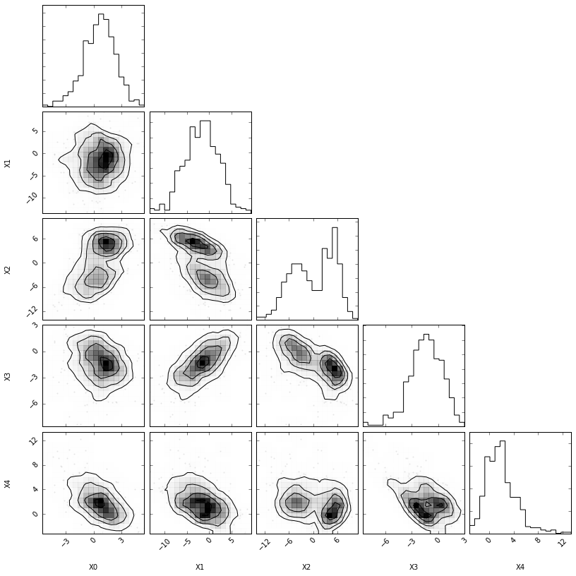
# Plot the data
import corner
fig = corner.corner(X_true, bins=20, smooth=0.85, labels=["X0", "X1", "X2", "X3", "X4"])
#plt.savefig("fig3.pdf")

png

Exact likelihood setup

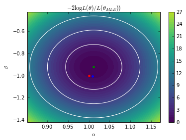
# Minimize the exact LR
from scipy.optimize import minimize

def nll_exact(theta, X):
    A.set_value(theta[0])
    B.set_value(theta[1])
    return (p0.nll(X) - p1.nll(X)).sum()

r = minimize(nll_exact, x0=[0, 0], args=(X_true,))
exact_MLE = r.x

print("Exact MLE =", exact_MLE)

Exact MLE = [ 1.01185168 -0.92213112]

# Exact contours
A.set_value(true_A)
B.set_value(true_B)

bounds = [(exact_MLE[0] - 0.16, exact_MLE[0] + 0.16),
          (exact_MLE[1] - 0.5, exact_MLE[1] + 0.5)]

As = np.linspace(*bounds[0], 100)
Bs = np.linspace(*bounds[1], 100)
AA, BB = np.meshgrid(As, Bs)
X = np.hstack((AA.reshape(-1, 1), BB.reshape(-1, 1)))

exact_contours = np.zeros(len(X))

i = 0
for a in As:
    for b in Bs:
        exact_contours[i] = nll_exact([a, b], X_true)
        i += 1

exact_contours = 2. * (exact_contours - r.fun)

plt.contour(As, Bs, exact_contours.reshape(AA.shape).T, 
            levels=[chi2.ppf(0.683, df=2), 
                    chi2.ppf(0.9545, df=2),
                    chi2.ppf(0.9973, df=2)], colors=["w"])
plt.contourf(As, Bs, exact_contours.reshape(AA.shape).T, 50, vmin=0, vmax=30)
cb = plt.colorbar()

plt.plot([true_A], [true_B], "r.", markersize=8)
plt.plot([exact_MLE[0]], [exact_MLE[1]], "g.", markersize=8)
#plt.plot([gp_MLE[0]], [gp_MLE[1]], "b.", markersize=8)

plt.axis((*bounds[0], *bounds[1]))
plt.xlabel(r"$\alpha$")
plt.ylabel(r"$\beta$")

#plt.savefig("fig4a.pdf")
plt.show()

png

Likelihood-free setup

In this example we will build a parametrized classifier $s(x; \theta_0, \theta_1)$ with $\theta_1$ fixed to $(\alpha=0, \beta=0)$.

# Build classification data
from carl.learning import make_parameterized_classification

bounds = [(-3, 3), (-3, 3)]

X, y = make_parameterized_classification(
    p0, p1,
    1000000, 
    [(A, np.linspace(*bounds[0], num=30)), 
     (B, np.linspace(*bounds[1], num=30))],
    random_state=1)

# Train parameterized classifier
from carl.learning import as_classifier
from carl.learning import make_parameterized_classification
from carl.learning import ParameterizedClassifier
from sklearn.neural_network import MLPRegressor
from sklearn.pipeline import make_pipeline
from sklearn.preprocessing import StandardScaler
from sklearn.model_selection import RandomizedSearchCV

clf = ParameterizedClassifier(
    make_pipeline(StandardScaler(), 
                  as_classifier(MLPRegressor(learning_rate="adaptive", 
                                             hidden_layer_sizes=(40, 40),
                                             tol=1e-6,
                                             random_state=0))),
    [A, B])
clf.fit(X, y)

For the scans and Bayesian optimization we construct two helper functions.

from carl.learning import CalibratedClassifierCV
from carl.ratios import ClassifierRatio

def vectorize(func):
    def wrapper(X):
        v = np.zeros(len(X))

        for i, x_i in enumerate(X):
            v[i] = func(x_i)

        return v.reshape(-1, 1)

    return wrapper

def objective(theta, random_state=0):    
    print(theta)

    # Set parameter values   
    A.set_value(theta[0])
    B.set_value(theta[1])

    # Fit ratio
    ratio = ClassifierRatio(CalibratedClassifierCV(
        base_estimator=clf, 
        cv="prefit",  # keep the pre-trained classifier
        method="histogram", bins=50))

    X0 = p0.rvs(n_samples=250000)
    X1 = p1.rvs(n_samples=250000, random_state=random_state)
    X = np.vstack((X0, X1))
    y = np.zeros(len(X))
    y[len(X0):] = 1

    ratio.fit(X, y)

    # Evaluate log-likelihood ratio
    r = ratio.predict(X_true, log=True)
    value = -np.mean(r[np.isfinite(r)])  # optimization is more stable using mean
                                         # this will need to be rescaled by len(X_true)    

    return value

from GPyOpt.methods import BayesianOptimization
bounds = [(-3, 3), (-3, 3)]
solver = BayesianOptimization(vectorize(objective), bounds)
solver.run_optimization(max_iter=50, true_gradients=False)

approx_MLE = solver.x_opt
print("Approx. MLE =", approx_MLE)

Approx. MLE = [ 1.01455539 -0.90202743]

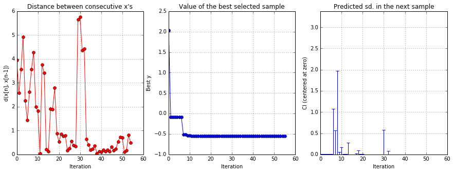
solver.plot_acquisition()

png

solver.plot_convergence()

png

# Minimize the surrogate GP approximate of the approximate LR
def gp_objective(theta):
    theta = theta.reshape(1, -1)
    return solver.model.predict(theta)[0][0]

r = minimize(gp_objective, x0=[0, 0])
gp_MLE = r.x

print("GP MLE =", gp_MLE)

GP MLE = [ 1.00846361 -1.00438228]

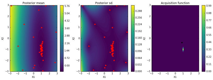
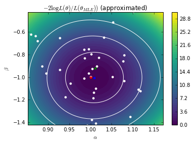
Here we plot the posterior mean of the Gaussian Process surrogate learned by the Bayesian Optimization algorithm.

# Plot GP contours
A.set_value(true_A)
B.set_value(true_B)

bounds = [(exact_MLE[0] - 0.16, exact_MLE[0] + 0.16),
          (exact_MLE[1] - 0.5, exact_MLE[1] + 0.5)]

As = np.linspace(*bounds[0], 100)
Bs = np.linspace(*bounds[1], 100)
AA, BB = np.meshgrid(As, Bs)
X = np.hstack((AA.reshape(-1, 1), BB.reshape(-1, 1)))

from scipy.stats import chi2
gp_contours, _= solver.model.predict(X)
gp_contours = 2. * (gp_contours - r.fun) * len(X_true)  # Rescale

cs = plt.contour(As, Bs, gp_contours.reshape(AA.shape), 
                 levels=[chi2.ppf(0.683, df=2), 
                         chi2.ppf(0.9545, df=2),
                         chi2.ppf(0.9973, df=2)], colors=["w"])
plt.contourf(As, Bs, gp_contours.reshape(AA.shape), 50, vmin=0, vmax=30)
cb = plt.colorbar()

plt.plot(solver.X[:, 0], solver.X[:, 1], 'w.', markersize=8)
plt.plot([true_A], [true_B], "r.", markersize=8)
plt.plot([exact_MLE[0]], [exact_MLE[1]], "g.", markersize=8)
plt.plot([gp_MLE[0]], [gp_MLE[1]], "b.", markersize=8)

plt.axis((*bounds[0], *bounds[1]))
plt.xlabel(r"$\alpha$")
plt.ylabel(r"$\beta$")

#plt.savefig("fig4b.pdf")
plt.show()

png

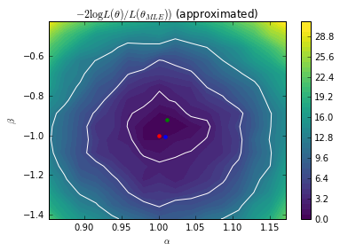
Finally, we plot the approximate likelihood from a grid scan. Statistical fluctuations in the calibration lead to some noise in the scan. The Gaussian Process surrogate above smooths out this noise providing a smoother approximate likelihood.

# Contours of the approximated LR
A.set_value(true_A)
B.set_value(true_B)

bounds = [(exact_MLE[0] - 0.16, exact_MLE[0] + 0.16),
          (exact_MLE[1] - 0.5, exact_MLE[1] + 0.5)]

As = np.linspace(*bounds[0], 16)
Bs = np.linspace(*bounds[1], 16)
AA, BB = np.meshgrid(As, Bs)
X = np.hstack((AA.reshape(-1, 1),
               BB.reshape(-1, 1)))

approx_contours = np.zeros(len(X))

i = 0
for a in As:    
    for b in Bs:
        approx_contours[i] = objective([a, b]) 
        i += 1

approx_contours = 2. * (approx_contours - approx_contours.min()) * len(X_true)

plt.contour(As, Bs, approx_contours.reshape(AA.shape).T, 
            levels=[chi2.ppf(0.683, df=2), 
                    chi2.ppf(0.9545, df=2),
                    chi2.ppf(0.9973, df=2)], colors=["w"])
plt.contourf(As, Bs, approx_contours.reshape(AA.shape).T, 50, vmin=0, vmax=30)
plt.colorbar()

plt.plot([true_A], [true_B], "r.", markersize=8)
plt.plot([exact_MLE[0]], [exact_MLE[1]], "g.", markersize=8)
plt.plot([gp_MLE[0]], [gp_MLE[1]], "b.", markersize=8)

plt.axis((*bounds[0], *bounds[1]))
plt.xlabel(r"$\alpha$")
plt.ylabel(r"$\beta$")

#plt.savefig("fig4c.pdf")
plt.show()

png

Index

Sub-modules

Notebooks

Parameterized inference from multidimensional data

Exact likelihood setup

Likelihood-free setup